Ingesting Dataset to H3

Raster to H3

The fused package includes functionality to automate the ingestion of raster data to an H3 dataset, through fused.h3.run_ingest_raster_to_h3().

In the following example, we will illustrate the usage of this function by ingesting a small Digital Elevation Model (DEM) file for the New York City region, available at "s3://fused-asset/data/nyc_dem.tif" (see in File Explorer).

The basic ingestion can be triggered from Workbench by running the following UDF:

@fused.udf
def udf():
    src_path = "s3://fused-asset/data/nyc_dem.tif"
    output_path = "s3://fused-users/fused/joris/nyc_dem_h3/"  # <-- update this path

    # run the ingestion process
    result_extract, result_partition = fused.h3.run_ingest_raster_to_h3(
        src_path, 
        output_path, 
        metrics=["avg"],
    )

    # verify that the ingestion finished succesfully,
    # and if not, print the error to help debugging
    if not result_extract.all_succeeded():
        print(result_extract.errors())
    if result_partition is not None and not result_partition.all_succeeded():
        print(result_partition.errors())

What is required to run this:

• src_path: A raster file path or list of file paths on S3 (e.g. a TIFF file, any raster format readable by GDAL)
• output_path: Specify a writeble location on S3 as the output directory
• metrics: Specify the metrics to compute per H3 cell: typically, multiple multiple pixel values from the input raster data will be used to calculate the value for a certain H3 cell. In this case of a DEM, we want the average pixel value (metrics=["avg"]).

Important to understand is that the run_ingest_raster_to_h3 function will run multiple UDFs under the hood to perform the separate steps of the ingestion process in parallel. Therefore, the above UDF itself does not need much resources (the heavy lifting is done in the UDF runs it spawns) but can take longer than the 2-min limit of realtime UDF runs.

For this small example, it runs fine on realtime. But for larger data, we will typically run this main UDF using a "small" batch instance.

@fused.udf(instance_type="small")
def udf():
    src_path = "s3://fused-asset/data/nyc_dem.tif"
    ...

What data did it create?

The run_ingest_raster_to_h3 function will write a set of files to the specified output directory:

• A number of Parquet files with the actual ingested data (577234808489377791.parquet in the example, but typically this will be multiple files)
• A single _sample metadata file, with information about the files and chunks that can help speed up reading a subset of the data.
• Overview files in the /overview sub-directory, such as hex3.parquet for the overview at H3 resolution 3.

For the NYC DEM example, this looks like:

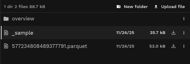
See an example of the ingested elevation data in File Explorer.

The data file looks like (s3://fused-asset/hex/nyc_dem/577234808489377791.parquet):

The overview file at resolution 7 looks like (s3://fused-asset/hex/nyc_dem/overview/hex7.parquet)

Each of the files include a "hex" column with the H3 cell ids at a specific resolution, and one or more columns derived from the raster data (in this case "data_avg" with the average height in the H3 cell).

Additionally, the data files include a "source_url" (source raster files) and "res" (H3 resolution) column. The overview files include a "lat"/"lng" column with the center of the H3 cell.

Reading and visualizing the H3 dataset

Both the data and overview files are Parquet files that can be read individually by any tool supporting the Parquet format. To make this easier, the example below uses the read_h3_dataset utility, that will automatically choose between reading a subset of actual data files vs overview files based on the viewport (bounds).

Reading the data for the NYC DEM example:

@fused.udf
def udf(
    bounds: fused.types.Bounds = [-74.556, 40.400, -73.374, 41.029],  # Default to full NYC
    res: int = None,
):
    path = "s3://fused-users/fused/joris/nyc_dem_h3/"

    utils = fused.load("https://github.com/fusedio/udfs/tree/dd40354/community/joris/Read_H3_dataset/")
    df = utils.read_h3_dataset(path, bounds, res=res)

    print(df.head())
    return df

                  hex   data_avg
0  617733120275513343   9.590167
1  617733120275775487  -2.473003
2  617733120276037631  14.483934
3  617733120276299775  -2.473003
4  617733120277086207  19.336820

We can visualize the data with DeckGL using the map_utils helper:

Standalone map UDF

@fused.udf
def udf(
    bounds: fused.types.Bounds = [-74.556, 40.400, -73.374, 41.029],  # Default to full NYC
    res: int = 9,
):
    path = "s3://fused-users/fused/joris/nyc_dem_h3/"

    utils = fused.load("https://github.com/fusedio/udfs/tree/dd40354/community/joris/Read_H3_dataset/")
    df = utils.read_h3_dataset(path, bounds, res=res)

    map_utils = fused.load("https://github.com/fusedio/udfs/tree/dd40354/community/milind/map_utils")

    config = {
        "hexLayer": {
            "@@type": "H3HexagonLayer",
            "filled": True,
            "pickable": True,
            "extruded": False,
            "opacity": 0.25,
            "getHexagon": "@@=properties.hex",
            "getFillColor": {
                "@@function": "colorContinuous",
                "attr": "data_avg",
                "domain": [0, 400],
                "steps": 20,
                "colors": "BrwnYl"
            }
        }
    }
    return map_utils.deckgl_hex(
        df, 
        config=config
    )

Specifying the metrics

In the basic DEM example above, we specified metrics=["avg"] to get the average height for each H3 cell.

In general, when converting the raster data to H3, an H3 cell can cover (partially) multiple pixels from the raster, and thus an aggregation is needed to calculate the resulting data point for the given H3 cell.

The type of aggregation best suited will depend on the kind of raster data:

• "cnt": for raster with discrete or categorical pixel values, e.g. as land use data, specify metric="cnt" to get a count per category for each H3 cell. This results in a "data" column with the category, a "cnt" column with the count for that category, and a "cnt_total" column with a sum of the counts per H3 cell (which allows to calculate the fraction of the H3 cell that is covered by a certain category).
• "avg": for raster data where each pixel represents the average value for that area, e.g. temperate, elevation or population density, the average gets preserved when converting to H3 cell areas (using a weighted average).
• "sum": for raster data where each pixel represents the total of the variable for that area, e.g. population counts, use the sum metric to preserve sums.

In addition, also the "min", "max" and "stddev" metrics are supported to calculate the minimum, maximum and standard deviation, respectively, of the pixel values covered by the H3 cell. Those metrics can be combined with calculating sums or averages, e.g. metrics=["avg", "min", "max"], while the "cnt" metric cannot be combined with any other metric, currently.

While the H3 cells at the data resolution might not cover that many pixel values (by default a resolution is chosen that matches the pixel area as close as possible), but note that those aggregations are also used for creating the overview files when aggregating the higher resolution H3 cells to lower resolution data.

Counting raster values (metrics=cnt)

For raster with discrete or categorical pixel values, e.g. as land use data, the "cnt" metric will count the number of occurences per catgory for each H3 cell.

This results in a "data" column with the category (i.e. original pixel values), a "cnt" column with the count for that category, and a "cnt_total" column with a sum of the counts per H3 cell (which allows to easily calculate the fraction of the H3 cell that is covered by a certain category).

Illustrating this with an example of ingested Cropland Data Layer (CDL) data, the resulting dataset looks like:

Code

@fused.udf
def udf(
    bounds: fused.types.Bounds = [-73.983, 40.763, -73.969, 40.773],  # Default to a small area in NYC
    res: int = None,
):
    # Cropland Data Layer (CDL) data, crop-specific land cover data layer
    # provided by the USDA National Agricultural Statistics Service (NASS).
    # Ingested using the "cnt" metric, counting the occurence of the land cover classes
    path = "s3://fused-asset/hex/cdls_v8/year=2024/"

    utils = fused.load("https://github.com/fusedio/udfs/tree/79f8203/community/joris/Read_H3_dataset")
    df = utils.read_h3_dataset(path, bounds, res=res)

    print(df.head())
    return df

                  hex  data  cnt  cnt_total
0  626740321835323391   122   12         14
1  626740321835323391   123    1         14
2  626740321835323391   121    1         14
3  626740321835327487   122    9         17
4  626740321835327487   121    4         17

Important to note: each H3 cell id can occur multiple times in the data in this case, because we have one row per category ("data") that occurs in that specific H3 cell.

In the example above, you can see the first H3 cell (626740321835323391) occuring 3 times, having counts for three categories (121, 122, 123).

Aggregating raster values (metrics=avg, sum, min, etc.)

When specifying one or more of the non-count metrics ("sum", "avg", "min", "max", "stddev"), a single value is obtained for each H3 cell by aggregating the pixel values using that metric.

This results in columns named "data_<metric>".

Illustrating this with the example of the ingested NYC DEM data, the resulting dataset looks like:

Code

@fused.udf
def udf(
    bounds: fused.types.Bounds = [-73.983, 40.763, -73.969, 40.773],  # Default to a small area in NYC
    res: int = None,
):
    # Ingested NYC DEM using the "avg" metric
    path = "s3://fused-asset/hex/nyc_dem/"

    utils = fused.load("https://github.com/fusedio/udfs/tree/79f8203/community/joris/Read_H3_dataset")
    df = utils.read_h3_dataset(path, bounds, res=res)

    print(df.head())
    return df

                  hex   data_avg
0  617733122581069823  78.822576
1  617733122610954239  78.225562
2  617733123866886143  47.372763
3  617733123867410431  55.030614
4  617733123871080447  74.679518

In this case, we have always one row per H3 cell id (in contrast to ingested data using the "cnt" metric).

H3 resolution levels

The run_ingest_raster_to_h3 function allows to specify the H3 resolution for different aspects of the ingested data through the res, file_res, chunk_res, overview_res, and overview_chunk_res.

Resolution of the data (res)

The main H3 resolution to specify is the resolution of the H3 cells in "hex" column in the output data. The raster data are converted to a grid of H3 cells at this resolution.

By default (if left unspecified), the resolution is inferred from the raster data. Using the resolution of the raster input, it chooses an H3 resolution with a cell size that is as close as possible to but larger than the pixel size (at the center of the raster). For example, this inference gives a resolution of 11 for a raster with pixel size of 30x30m, and a resolution of 10 for a raster with pixel size of 90x90m.

H3 Resolution (res)	Average Hex Area (m²)	Average Hex Edge Length (m)	Pixel Size Equivalent (m, √ avg hex area)	Common Raster Dataset Example
0	4,357,449,416,078	1,281,256	2,087,465
1	609,788,441,794	483,057	780,889
2	86,801,780,399	182,513	294,621
3	12,393,434,655	68,979	111,325
4	1,770,347,654	26,072	42,075	ERA 5 (0.25deg ~ 27km at Equator)
5	252,903,858	9,854	15,903
6	36,129,062	3,725	6,011
7	5,161,293	1,406	2,272
8	737,328	531	859
9	105,333	201	325	Modis Vegetation Index (250m)
10	15,048	76	123
11	2,150	29	46	Landsat Collection 2 (30m)
12	307.1	10.8	17.5	Sentinel-2 (10m)
13	43.9	4.1	6.6
14	6.3	1.5	2.5	USGS LiDAR DEM (1m)
15	0.9	0.6	0.9

Notes:

• Values are approximate (area and edge length slightly vary by latitude/longitude).
• "Pixel Size Equivalent" is the square root of the average hex area, to aid raster/pixel comparison.

For more details see the H3 Cell Counts Stats page.

Dataset partitioning (file_res and chunk_res)

The ingested data as Parquet dataset is spatially partitioned. In this case, this means that the data is sorted by the "hex" column (the H3 cells at resolution res), and further splitted into multiple files and chunks.

To determine how to split the dataset in multiple files, a lower H3 resolution is used (file_res). By default, this is inferred based on the resolution res of the data, targetting to have individual files of around 100MB up to 1GB in size (approximately, and assuming there is one row per H3 cell).

Each Parquet file is further chunked into "row groups", and by default another H3 resolution is used to determine this level of splitting (chunk_res). By default, this is again inferred from the data resolution, targetting chunks of around 1 million rows (assuming one row per H3 cell and full coverage).

Example: for a data resolution of 10, by default a file resolution of 0 and chunk resolution of 3 will be used. The file resolution of 0 results in a maximum of 122 files for a global dataset. The chunk resolution of 3 gives a maximum of 343 (7^3) row groups, and for a dataset with full coverage and one row per H3 cell at the data resolution, approximately 820,000 rows (7^(10-3)) in a single file.

The optimal values for those resolutions will of course depend on the characteristics of the input data and ingestion (raster resolution, extent, cardinality of the categories, which metrics are used, etc), and the desired trade off for file and chunk sizes (in general, smaller chunks improve the speed of selective queries (i.e. reading a small (spatial) subset) but slow down queries that have to scan the whole file). It is therefore always possible to override the defaults by specifying the keywords in the run_ingest_raster_to_h3() call.

Two special cases to mention:

• If you have a smaller dataset, it might not be worth splitting into multiple files. In that case, specify file_res=-1 to request a single output file.
• The chunks can also be determined by specifying an exact size (number of rows), instead of specifying an H3 resolution (chunk_res), using the max_rows_per_chunk keyword instead.

Overview resolutions (overview_res)

In addition to the actual data files at resolution res, the ingestion process also produces "overview" files in the /overview/ sub-directory. Those files each have an aggregated version of the full dataset at a lower overview resolution (aggregated using the same metric as the actual data).

The files use the naming pattern of hex<res>.parquet, e.g. /overview/res3.parquet for the overview file at resolution 3.

By default, overviews are created for H3 resolutions 3 to 7 (or capped at res - 1 if data resolution is lower than 8). But you can specify a list of resolutions for which to create overview files by specifying the overview_res keyword.

@fused.udf(instance_type="small")
def udf():
    src_path = "s3://fused-asset/data/nyc_dem.tif"
    output_path = "s3://fused-users/fused/joris/nyc_dem_h3/"  # <-- update this path

    result_extract, result_partition = fused.h3.run_ingest_raster_to_h3(
        src_path, 
        output_path, 
        metrics=["avg"],
        overview_res=[7,6,5,4,3],   # Setting up overviews for resolutions 7 through 3
    )

This would create the following overview files:

File Path	Size
s3://.../nyc_dem_h3/overview/hex3.parquet	36.9 kB
s3://.../nyc_dem_h3/overview/hex4.parquet	36.9 kB
s3://.../nyc_dem_h3/overview/hex5.parquet	37.1 kB
s3://.../nyc_dem_h3/overview/hex6.parquet	37.4 kB
s3://.../nyc_dem_h3/overview/hex7.parquet	41.1 kB

Also the overview files are chunked in row groups. By default it uses a chunk resolution of overview_res - 5 (i.e. if the res is 11, the default chunk resolution for the overview files will be 6), but this default can be overridden with the overview_chunk_res keyword, or by specifying a max_rows_per_chunk.

Ingesting multiple files

Single file

@fused.udf
def udf():
    src_path = "s3://fused-asset/data/nyc_dem.tif"
    output_path = "s3://fused-users/fused/joris/nyc_dem_h3/"  # <-- update this path

result_extract, result_partition = fused.h3.run_ingest_raster_to_h3(
    src_path, 
    output_path, 
    metrics=["avg"],
)

Directory of files

@fused.udf
def udf():
    src_path = fused.api.list("s3://copernicus-dem-90m/")
    print(len(src_path))
    output_path = "s3://fused-users/fused/joris/cop90m_dem/"  # <-- update this path

result_extract, result_partition = fused.h3.run_ingest_raster_to_h3(
    src_path, 
    output_path, 
    metrics=["avg"],
)

Multiple file paths

Ingestion works with any hosted raster data

Your file paths do not need to be hosted on the Fused S3 bucket (i.e. you can ingest data from any S3 bucket or hosted location).

@fused.udf
def udf():
    dem_listing = [
        "s3://copernicus-dem-90m/Copernicus_DSM_COG_30_N51_00_E004_00_DEM/Copernicus_DSM_COG_30_N51_00_E004_00_DEM.tif",
        "s3://copernicus-dem-90m/Copernicus_DSM_COG_30_N51_00_E005_00_DEM/Copernicus_DSM_COG_30_N51_00_E005_00_DEM.tif",
        "s3://copernicus-dem-90m/Copernicus_DSM_COG_30_N52_00_E004_00_DEM/Copernicus_DSM_COG_30_N52_00_E004_00_DEM.tif",
        "s3://copernicus-dem-90m/Copernicus_DSM_COG_30_N52_00_E005_00_DEM/Copernicus_DSM_COG_30_N52_00_E005_00_DEM.tif",
    ]
    output_path = "s3://fused-users/fused/joris/copernicus-dem-90m/"  # <-- update this path

    result_extract, result_partition = fused.h3.run_ingest_raster_to_h3(
        dem_listing,
        output_path,
        metrics=["avg"],
    )
    ...

For ingesting the full dataset, you can create the list of input paths by listing the online S3 bucket and filtering for the desired TIFF files.

Controlling the ingestion execution

The run_ingest_raster_to_h3() function will run multiple UDFs under the hood to perform the separate steps of the ingestion process in parallel.

The different steps:

• "extract": extract the pixels values and assign to H3 cells in chunks
• "partition": combine the chunked, extracted data per partition (file), and prepare metadata and overview files
• create the metadata _sample file (with information about the file and chunk bounding boxes)
• "overview": create the combined overview files

The extract, partition and overview steps are each run in parallel using fused.submit().

By default, each of those steps are first tried as realtime UDF runs, and retry any failed runs using "large" batch instances (e.g. the realtime run can fail because the chunk takes too much time to process or the data is too big to fit in a small realtime instance).

You can override this default behavior by specifying the engine and/or instance_type keyword to specify the exact instance you want to use for the steps.

Further keywords of fused.submit() can be specified to tweak the exact execution of the steps. For example, specify max_workers to indicate a larger number of parallel workers to use.

Running ingestion on GCP

Fused can run the ingestion fully on GCP batch instances (realtime execution will still be done on AWS at this point however), if they are available in your environment:

@fused.udf(instance_type="c2-standard-4") # <- using GCP instance to orchestrate the ingestion
def udf():

    src_path = "s3://fused-asset/data/nyc_dem.tif"
    output_path = "s3://fused-users/fused/joris/nyc_dem_h3/"  # <-- update this path

    result_extract, result_partition = fused.h3.run_ingest_raster_to_h3(
        src_path, 
        output_path, 
        metrics=["avg"],                # DEM, so using avg 
        instance_type="c2-standard-60", # Using large GCS for actual compute steps
    )

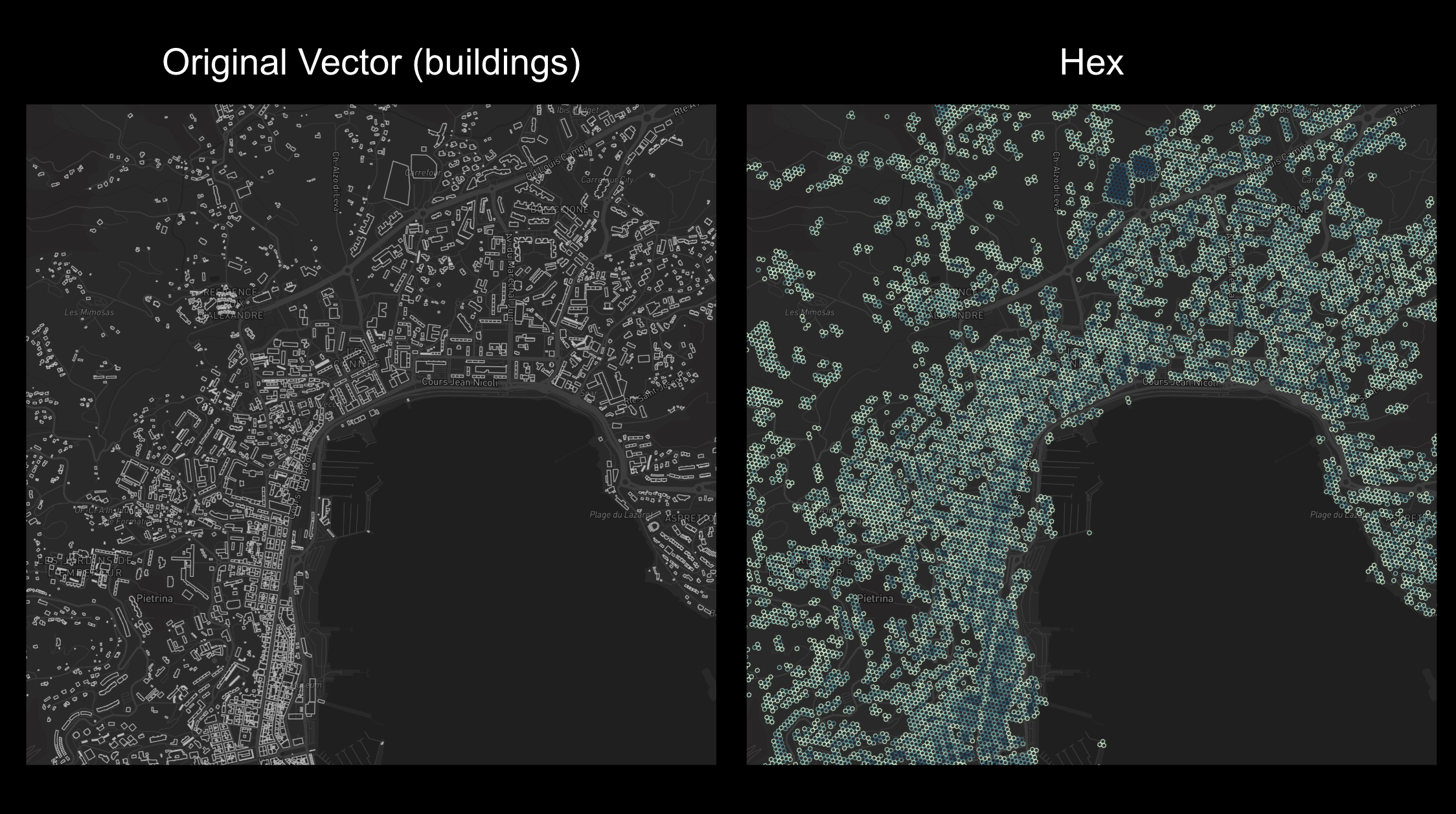
Vector to Hex

Example of ingesting a release of the Overture Building dataset to H3 hexagons:

release = '2025-01-22-0'

args = [{'input_path': f's3://us-west-2.opendata.source.coop/fused/overture/{release}/theme=buildings/type=building/',
         'output_path': f's3://fused-users/fused/max/overture_overview/{release}/', # <-- replace this with your own S3 bucket 
         'hex_res': 11}]

In this example we'll be simply counting the number of buildings per hexagon.

Overture_Hexify = fused.load("https://github.com/fusedlabs/fusedudfs/tree/main/Overture_Hexify/")
j = Overture_Hexify(arg_list=args)

j.run_remote(instance_type='r5.16xlarge', disk_size_gb=999)

Reading the ingested data becomes a lot simpler & faster:

Code

common = fused.load("https://github.com/fusedio/udfs/blob/main/public/common/")
@fused.udf
def udf(bounds: fused.types.Bounds = [-122.71963771127753,36.53196328805067,-120.70395948802646,38.082911654639275]):
    res = bounds_to_res(bounds)
    print(res)
    releases = ['2024-02-15-alpha-0', '2024-03-12-alpha-0', '2024-08-20-0', '2024-09-18-0', '2024-10-23-0', '2024-11-13-0', '2024-12-18-0', '2025-01-22-0', '2025-03-19-1', '2025-04-23-0', '2025-05-21-0']
    release1 = releases[-1]
    df1 = common.read_hexfile(bounds, f"s3://fused-users/fused/sina/overture_overview/{release1}/hex{res}.parquet", clip=True)

    return df1

@fused.cache
def bounds_to_res(bounds, res_offset=0, max_res=14, min_res=3):
    z = common.estimate_zoom(bounds)
    return max(min(int(3 + max(0, z - 3) / 1.7 + res_offset), max_res), min_res)